spotifyr is an R wrapper for pulling track audio features and other information from Spotify’s Web API in bulk. By automatically batching API requests, it allows you to enter an artist’s name and retrieve their entire discography in seconds, along with Spotify’s audio features and track/album popularity metrics. You can also pull song and playlist information for a given Spotify User (including yourself!).
CRAN version 2.2.3 (recommended)
install.packages('spotifyr')Development version
devtools::install_github('charlie86/spotifyr')First, set up a Dev account with Spotify to access their Web API here.
This will give you your Client ID and
Client Secret. Once you have those, you can pull your
access token into R with get_spotify_access_token().
The easiest way to authenticate is to set your credentials to the
System Environment variables SPOTIFY_CLIENT_ID and
SPOTIFY_CLIENT_SECRET. The default arguments to
get_spotify_access_token() (and all other functions in this
package) will refer to those. Alternatively, you can set them manually
and make sure to explicitly refer to your access token in each
subsequent function call.
Sys.setenv(SPOTIFY_CLIENT_ID = 'xxxxxxxxxxxxxxxxxxxxx')
Sys.setenv(SPOTIFY_CLIENT_SECRET = 'xxxxxxxxxxxxxxxxxxxxx')

access_token <- get_spotify_access_token()For certain functions and applications, you’ll need to log in as a
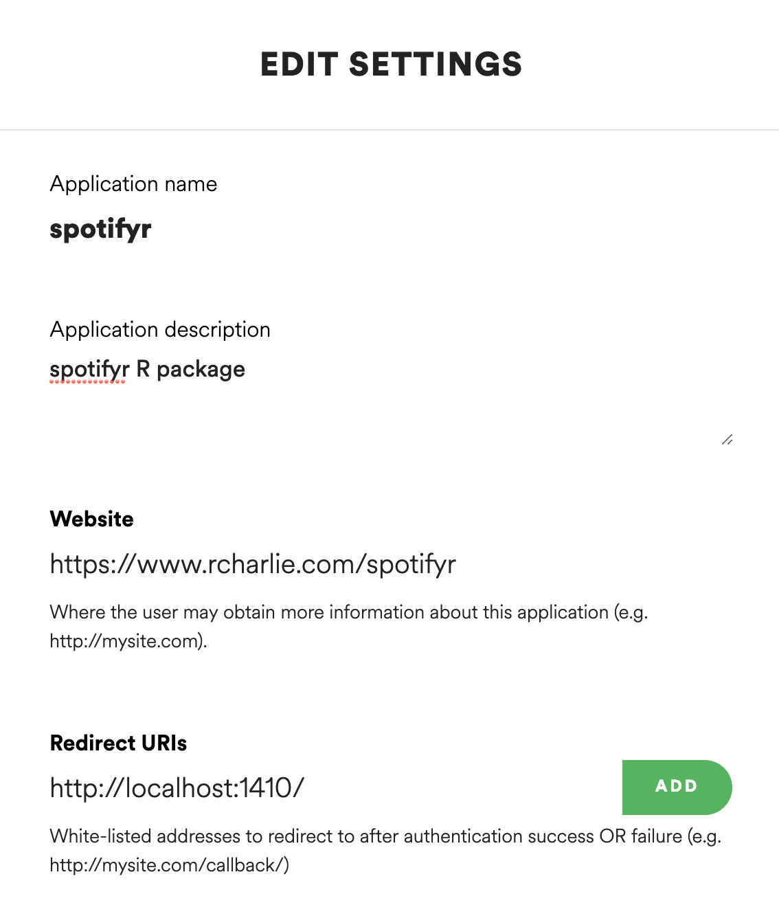
Spotify user. To do this, your Spotify Developer application needs to
have a callback url. You can set this to whatever you want that will
work with your application, but a good default option is
http://localhost:1410/ (see image below). For more
information on authorization, visit the offical Spotify
Developer Guide.

library(spotifyr)
beatles <- get_artist_audio_features('the beatles')library(dplyr)
library(purrr)
library(knitr)
beatles %>%
count(key_mode, sort = TRUE) %>%
head(5) %>%
kable()| key_mode | n |
|---|---|
| D major | 115 |
| C major | 111 |
| G major | 90 |
| A major | 80 |
| E major | 68 |
library(lubridate)
#> Warning: package 'lubridate' was built under R version 4.1.1

get_my_recently_played(limit = 5) %>%
    mutate(
        artist.name = map_chr(track.artists, function(x) x$name[1]),
        played_at = as_datetime(played_at)
        ) %>%
    select(
      all_of(c("track.name", "artist.name", "track.album.name", "played_at"))
      ) %>%
kable()| track.name | artist.name | track.album.name | played_at |
|---|---|---|---|
| Look For Me (I’ll Be Around) | Neko Case | Blacklisted | 2021-11-01 17:16:12 |
| Don’t Forget Me | Neko Case | Middle Cyclone | 2021-11-01 17:12:50 |
| Magpie to the Morning | Neko Case | The Worse Things Get, The Harder I Fight, The Harder I Fight, The More I Love You (Deluxe Edition) | 2021-11-01 17:09:42 |
| Margaret vs. Pauline | Neko Case | Fox Confessor Brings The Flood (Bonus Track Version) | 2021-11-01 17:06:45 |
| Runnin’ Out Of Fools | Neko Case | Blacklisted | 2021-11-01 17:03:52 |
get_my_top_artists_or_tracks(type = 'artists',
                             time_range = 'long_term',
                             limit = 5) %>%
    select(.data$name, .data$genres) %>%
    rowwise %>%
    mutate(genres = paste(.data$genres, collapse = ', ')) %>%
    ungroup %>%
kable()| name | genres |
|---|---|
| Japanese Breakfast | art pop, eugene indie, indie pop, philly indie |
| Balthazar | belgian indie, belgian rock, dutch indie, ghent indie |
| Haley Bonar | melancholia, stomp and holler |
| Angus & Julia Stone | australian indie folk, indie folk, stomp and holler |
| Buildings Breeding | indie fuzzpop |
get_my_top_artists_or_tracks(type = 'tracks',
                             time_range = 'short_term',
                             limit = 5) %>%
    mutate(
        artist.name = map_chr(artists, function(x) x$name[1])
        ) %>%
    select(name, artist.name, album.name) %>%
kable()| name | artist.name | album.name |
|---|---|---|
| Can’t Walk That Back | Tristen | Can’t Walk That Back |
| You’re Too Weird | Fruit Bats | Tripper |
| California (All the Way) | Luna | Bewitched |
| Don’t Blame Your Daughter (Diamonds) | The Cardigans | Super Extra Gravity (Remastered) |
| Born In The ’70s | Fruit Bats | Spelled In Bones |
My favorite audio feature has to be “valence,” a measure of musical positivity.
joy <- get_artist_audio_features('joy division')joy %>%
arrange(-valence) %>%
select(.data$track_name, .data$valence) %>%
head(5) %>%
kable()| track_name | valence |
|---|---|
| Passover - 2020 Digital Master | 0.946 |
| Passover - 2007 Remaster | 0.941 |
| Colony - 2020 Digital Master | 0.829 |
| Colony - 2007 Remaster | 0.808 |
| Atrocity Exhibition - 2020 Digital Master | 0.790 |
Now if only there was some way to plot joy…
library(ggplot2)
library(ggridges)

ggplot(
    joy,
    aes(x = valence, y = album_name)
    ) +
geom_density_ridges() +
theme_ridges() +
labs(title = "Joyplot of Joy Division's joy distributions",
     subtitle = "Based on valence pulled from Spotify's Web API with spotifyr")
The coolest thing about making this package has definitely been seeing all the awesome stuff other people have done with it. Here are a few examples:
Exploring the Spotify API with R: A tutorial for beginners, by a beginner, Mia Smith
Blue Christmas: A data-driven search for the most depressing Christmas song, Caitlin Hudon
Sente-se triste quando ouve “Amar pelos dois”? Não é o único (Do you feel sad when you hear “Love for both?” You’re not alone), Rui Barros, Rádio Renascença
Using Data to Find the Angriest Death Grips Song, Evan Oppenheimer
Hierarchical clustering of David Bowie records, Alyssa Goldberg
tayloR, Simran Vatsa
Please note that the spotifyr project is released with a Contributor Code of Conduct. By contributing to this project, you agree to abide by its terms.