The goal of ovbsa (omitted variable bias sensitivity
analysis) is to conduct sensitivity analysis of omitted variable bias in
linear econometrics models. For details see Basu (2025).
You can install the package ovbsa from CRAN with:
# uncomment this line
# install.packages("ovbsa")
You can install the development version of ovbsa from GitHub with:
# uncomment these lines
# install.packages("pak")
# pak::pak("dbasu-umass/ovbsa")The main functions in this package are:
bsal: this function conducts basic sensitivity
analysis (bsal) and reports the bias-adjusted estimate, the
bias-adjusted standard error and the bias-adjusted confidence interval
in a linear regression model;
saltr2: this function computes the probability of
the conclusion of the study being overturned using the total
R-squared-based analysis;
salpr2ncd: this function computes the probability of
the conclusion of the study being overturned using the partial
R-squared-based analysis without conditioning on the treatment
variable;
Let us first load the relevant libraries and then work through two examples.
library(ovbsa)
library(sensemakr)
#> See details in:
#> Carlos Cinelli and Chad Hazlett (2020). Making Sense of Sensitivity: Extending Omitted Variable Bias. Journal of the Royal Statistical Society, Series B (Statistical Methodology).library(ggplot2)In the examples we will use use the data set darfur from
the package sensemakr, which studies the effect of exposure
to violence on attitudes towards peace.
This is a basic example which shows you how to find the bias-adjusted
estimate, the bias-adjusted standard error and the bias-adjusted
confidence interval in a linear regression model. To use this function
the user needs to choose a benchmark covariate, values of the
sensitivity parameters kD and kY and the
significance level alpha for testing the null hypothesis
that the treatment effect is zero.
Here we choose the benchmark covariate as female,
kD=3, kY=3 and alpha=0.05
## basic example code
analysis1 <- ovbsa::bsal(
  kd=3,ky=3,alpha=0.05,data=darfur,
  outcome = "peacefactor",
  treatment = "directlyharmed",
  bnch_reg = "female",
  other_reg = c("village","age","farmer_dar","herder_dar",
                "pastvoted","hhsize_darfur")
)
Now, let us see the results.
(analysis1)
#>                        Case 1       Case 2
#> r2yd.x            0.021873093  0.021873093
#> r2dz.x            0.008040002  0.027492860
#> r2yz.dx           0.781414454  0.380969988
#> estimate          0.097315819  0.097315819
#> adjusted_estimate 0.045525612  0.029779889
#> adjusted_se       0.010924114  0.018566585
#> adjusted_lower_CI 0.024081595 -0.006666285
#> adjusted_upper_CI 0.066969628  0.066226063
Here Case 1 refers to the total R-squared-based approach; Case 2 refers to the partial R-squared-based approach without conditioning on the treatment variable.
Continuing with the previous example, we will now compute the
probability that taking account of omitted variable bias will overturn
the conclusion of the study. We will need to choose the significance
level alpha for testing the null hypothesis that the
treatment effect is zero, the mode (and median) k_kd of the
parameter kD, and the mode (and median) k_ky of the
parameter kY.
Here we choose alpha=0.05, k_kd=1, k_ky=1.
First, we will look at total R-squared based analysis:
# total r2-based analysis
res1 <- ovbsa::saltr2(
  alpha=0.05,data = darfur, outcome = "peacefactor",
  treatment = "directlyharmed", bnch_reg = "female",
  other_reg = c("village","age","farmer_dar","herder_dar",
                "pastvoted","hhsize_darfur"),
  N = 500, k_kd=1, k_ky=1
)
# probability
(res1$frac_prob_wt)
#> [1] 0.2582741
Second: we will see the partial R-squared based analysis without conditioning on the treatment variable:
res2 <- ovbsa::salpr2ncd(
  alpha=0.05,data = darfur, outcome = "peacefactor",
  treatment = "directlyharmed", bnch_reg = "female",
  other_reg = c("village","age","farmer_dar","herder_dar",
                "pastvoted","hhsize_darfur"),
  N = 500, k_kd=1, k_ky=1
)
# probability
(res2$frac_prob_wt)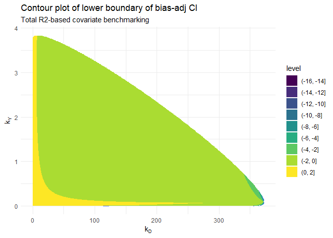
#> [1] 0.3118923The above functions used to compute the probability of a study’s conclusion being overturned implicitly used a contour plot of the boundary of the bias-adjusted confidence interval. The data is available as an output to be used by researchers to create that plot, if needed.
I will use the output of the total R-squared-based analysis to create
the contour plot. The data frame to construct the contour plot is
available as a data frame in res1$dataplot. For the contour
plot, we will need three variables from this data frame: X1
as the x-axis, X2 as the y-axis and Z3 as the
z-axis (value of the lower boundary of the bias-adjusted confidence
interval).
# the contour plot
ggplot(data = res1$dataplot, aes(X1, X2, z = Z3)) +
      geom_contour() +
      geom_contour_filled() +
      labs(
        title = "Contour plot of lower boundary of bias-adj CI",
        subtitle = "Total R2-based covariate benchmarking"
      ) +
      xlab(expression(k[D])) +
      ylab(expression(k[Y])) +
      theme_minimal()
#> Warning: Removed 96443 rows containing non-finite outside the scale range
#> (`stat_contour()`).
#> Warning: Removed 96443 rows containing non-finite outside the scale range
#> (`stat_contour_filled()`).
For easy reference, the following information about the relevant variables in the data frame should be noted while constructing contour plots like the one above:
when the unadjusted estimate is positive, use X1 as
the x-axis, X2 as the y-axis and Z3 as the
z-axis (value of the lower boundary of the bias-adjusted confidence
interval);
when the unadjusted estimate is negative, use X1 as
the x-axis, X2 as the y-axis and Z4 as the
z-axis (value of the lower boundary of the bias-adjusted confidence
interval).