oneinflThe R package oneinfl estimates one-inflated positive
Poisson (OIPP) and one-inflated zero-truncated (OIZTNB) regression
models. When count data are truncated so that \(y = 1,2,\dots\), it is also often inflated
at \(y=1\). The current standard model
for treating such data is the zero-truncated negative binomial (ZTNB)
model. ZTNB fails to account for excess 1s (or too few 1s), resulting in
biased and inconsistent estimators.
This readme illustrates oneinfl by reproducing and
extending the MedPar results in “One-inflated zero-truncated
count regression models” (Godwin, 2024).
Load the medpar data from the msme
package:
library(msme)
data(medpar)
df = medparformula <- los ~ white + died + type2 + type3 | white + died + type2 + type3
OIZTNB <- oneinfl(formula, df, dist="negbin")
OIPP <- oneinfl(formula, df, dist="Poisson")formula is the population model to be estimated,
variables that precede | link to the mean function and
variables that follow | link to one-inflation.
df is a data frame and dist="negbin" estimates
OIZTNB while dist="Poisson" estimates OIPP.
These are the current standard models for treating zero-truncated count data.
formula <- los ~ white + died + type2 + type3
ZTNB <- truncreg(formula, df, dist="negbin")
PP <- truncreg(formula, df, dist="Poisson")oneLRT extracts the log-likelihood and number of
parameters in any two models estimated by oneinfl or
truncreg. It returns the likelihood ratio test statistic
and its associated p-value. It can be used to test hypotheses
involving nested models.
Likelihood ratio test for overdispersion:
oneLRT(OIZTNB, OIPP)$LRTstat
[1] 3305.341
$pval
[1] 0We reject the null hypothesis of no overdispersion. Overdispersion is a well-developed topic that has led many to discard a Poisson model in favour of a negative binomial model. The principle extends to both truncated data (the ZTNB model vs. the PP model) and one-inflation (OIZTNB vs. OIPP).
Likelihood ratio test for one-inflation:
oneLRT(OIZTNB, ZTNB)$LRTstat
[1] 131.4165
$pval
[1] 0The LRT supports the presence of one-inflation (the null hypothesis is no one-inflation).
Godwin (2024) presents a Wald test for the presence of one-inflation.
Only a one-inflated model estimated by oneinfl is
needed.
oneWald(OIZTNB)$W
[1] 469.1062
$pval
[1] 0The Wald test also supports the presence of one-inflation.
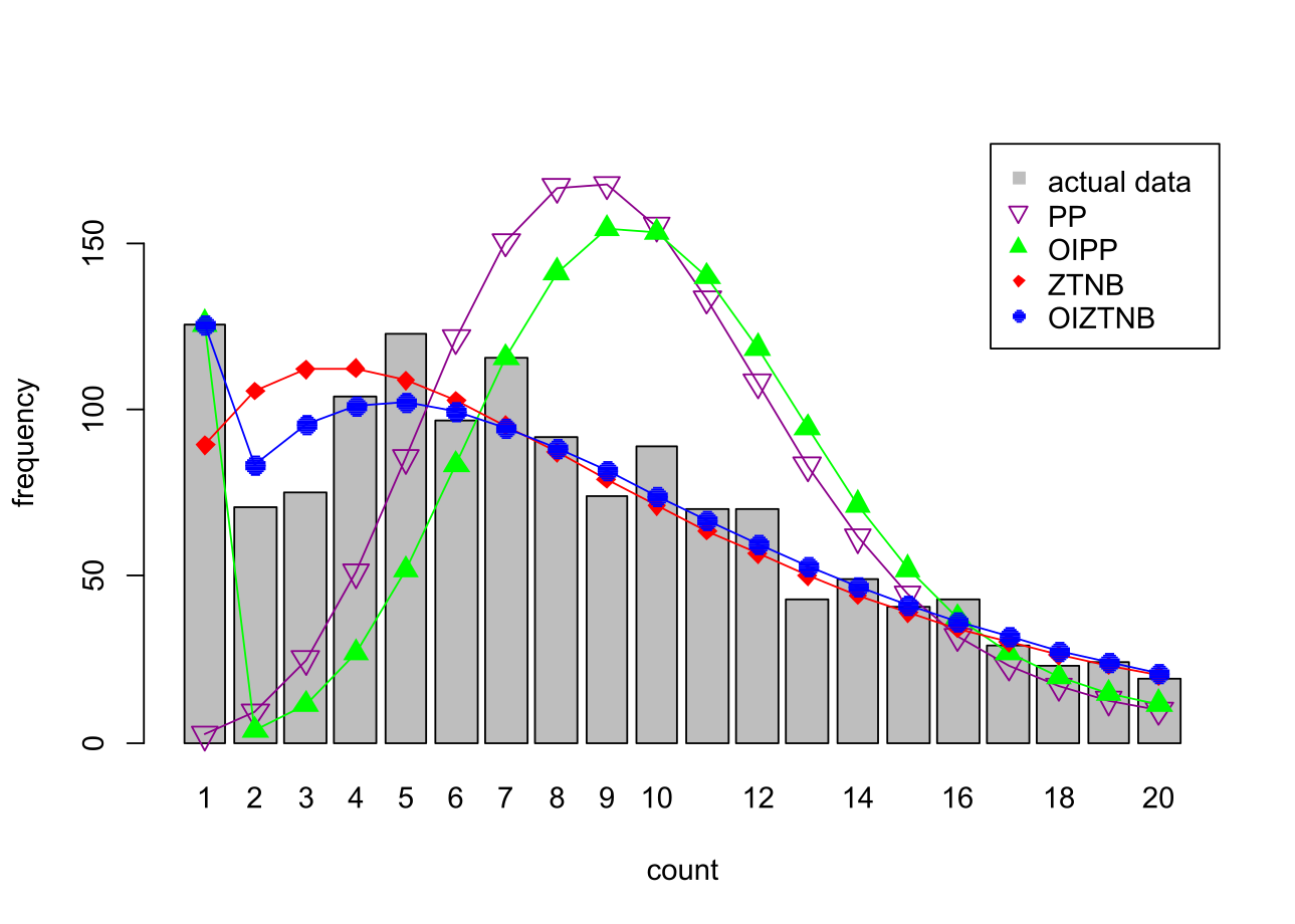
Plot all of the estimated models using:
oneplot(PP, OIPP, ZTNB, OIZTNB, data=data, maxpred=20, ylimit=180)which produces the following plot:
A custom S3 summary function for OIZTNB, OIPP, ZTNB, and PP models
estimated using oneinfl() or truncreg(),
provides output similar to standard uses of summary().
summary(OIZTNB)Call:
formula: los ~ white + died + type2 + type3 | white + died + type2 + type3
distribution: negbin
Coefficients (beta):
Estimate Std.Error z_value p.value
b(Intercept) 2.29913 0.07184 32.005 0.000e+00 ***
bwhite -0.09708 0.07138 -1.360 1.738e-01
bdied -0.06814 0.04492 -1.517 1.293e-01
btype2 0.23413 0.05349 4.377 1.204e-05 ***
btype3 0.75580 0.07884 9.586 0.000e+00 ***
Coefficients (gamma):
Estimate Std.Error z_value p.value
g(Intercept) -4.2002 0.5060 -8.300 0.00000 ***
gwhite 0.6594 0.4814 1.370 0.17075
gdied 2.3349 0.2359 9.899 0.00000 ***
gtype2 -0.5413 0.2829 -1.913 0.05569 .
gtype3 -0.7507 0.4472 -1.679 0.09324 .
alpha:
Estimate Std.Error z_value p.value
1 2.267 0.146 15.53 0 ***
Signif. codes: 0 `***' 0.001 `**' 0.01 `*' 0.05 `.' 0.1 ` ' 1
average one-inflation: 0.0416855179433309
average absolute one-inflation: 0.0680909723883016
Log-likelihood: -4671.06423844655For example, when the variable \(died = 1\), one-inflation increases significantly, but \(died\) otherwise does not effect los. Average one-inflation is 4.2% (there is an additional 0.042 probability that each person will stay only 1 day). Average absolute one-inflation is 0.068, meaning that some observations have one-deflation (e.g. when \(type2\) or \(type3\) equals 1).
To reproduce the results form Chapter 11.1 in Hilbe (2011), we summarize the ZTNB model using:
summary(ZTNB)Call:
formula: los ~ white + died + type2 + type3
distribution: negbin
Coefficients (beta):
Estimate Std.Error z_value p.value
b(Intercept) 2.3334 0.07499 31.115 0.000e+00 ***
bwhite -0.1318 0.07469 -1.765 7.755e-02 .
bdied -0.2512 0.04468 -5.622 1.889e-08 ***
btype2 0.2601 0.05529 4.704 2.550e-06 ***
btype3 0.7692 0.08259 9.314 0.000e+00 ***
alpha:
Estimate Std.Error z_value p.value
1 1.881 0.1034 18.19 0 ***
Signif. codes: 0 `***' 0.001 `**' 0.01 `*' 0.05 `.' 0.1 ` ' 1
Log-likelihood: -4736.77246562658 Taking exp(ZTNB$beta) gives the incident risk
ratios.
Since variables are typically linked to both the rate parameter \(\lambda\) and the one-inflating parameter \(\omega\), tests of overall significance are joint hypotheses. Testing the overall significance of the variable \(white\) for example, use:
signifWald(OIZTNB, "white")$W
[1] 3.725885
$pval
[1] 0.1552153The p-value of 0.155 suggests that the variable does not have a significant effect on \(los\), which is contrary to the standard ZTNB model.
Marginal effects can be estimated at the default “average effects” (the marginal effect is estimated at each observation and averaged over all observations):
margins(OIZTNB, df)Call:
formula: los ~ white + died + type2 + type3 | white + died + type2 + type3
distribution: negbin
Marginal effects:
Marginal.effects Std.Error z_value p.value
white -1.258 0.7344 -1.713 8.668e-02 .
died -2.189 0.3964 -5.522 3.343e-08 ***
type2 2.575 0.5875 4.382 1.174e-05 ***
type3 10.142 1.4663 6.917 4.616e-12 ***
Signif. codes: 0 `***' 0.001 `**' 0.01 `*' 0.05 `.' 0.1 ` ' 1these marginal effects can be compared to other models estimated by
oneinfl, for example using:
margins(ZTNB, data)Marginal effects can be estimated at the “effect at means” (the data is averaged before evaluating the marginal effect):
margins(OIZTNB, data, at = "EM")or at a representative case:
margins(OIZTNB, data, at = list(white = 0, died = 0, type2 = 0, type3 = 0))Generate predicted counts from an OIZTNB model:
pred(OIZTNB, data)or from any of the four models:
pred(ZTNB, data)Random variates can be generated using roipp(b, g, X, Z)
and roiztnb(b, g, a, X, Z). For example:
n <- 100
X <- data.frame(rep(1, n), rnorm(n))
Z <- X
roipp(b=c(0, 0), g=c(0, 0), X, Z)
roiztnb(b=c(0, 0), g=c(0, 0), a=1, X, Z)To evaluate \(E[y_i | \hat{\theta_i}]\) use:
predict(model = OIZTNB, data = medpar)for example.