![]()
![]()
In cheapr, ‘cheap’ means fast and memory-efficient, and that’s exactly the philosophy that cheapr aims to follow.
You can install cheapr like so:
install.packages("cheapr")or you can install the development version of cheapr:
remotes::install_github("NicChr/cheapr")cheapr is primarily an extension to R for developers that want to write clean, fast and safe code without sacrificing any one of these core design principles.
Some common R operations that cheapr can do much faster and more efficiently include:
Handling NA values very efficiently
Counting, finding, removing and replacing scalar values
Type-stable one-way casting and common-casting
Combining vectors
Creating and manipulating factors
Pasting strings
Creating multiple sequences in a vectorised way
Sub-setting vectors and data frames efficiently
Safe, flexible and fast greatest common divisor and lowest common multiple
Lags/leads
integer64 support
In-memory Math (no copies, vectors updated by reference)
Summary statistics
Counts
Modifying lists
Recycling
Binning of continuous data
NALet’s first load the required packages
library(cheapr)
library(bench)
Because R mostly uses vectors and vectorised operations, this means that there are few scalar-optimised operations.
cheapr provides tools to efficiently count, find, replace and remove scalars.
# Setup data with NA values
set.seed(42)
x <- sample(1:5, 30, TRUE)
x <- na_insert(x, n = 7)

counts(x) # Fast counts
#>   key count
#> 1   1     6
#> 2   5     4
#> 3  NA     7
#> 4   2     6
#> 5   4     4
#> 6   3     3
NA functions
na_count(x)
#> [1] 7
na_rm(x)
#>  [1] 1 5 1 2 4 2 1 4 5 4 2 3 1 1 3 4 5 5 2 3 2 1 2
na_find(x)
#> [1]  4  8 11 15 22 24 26
na_replace(x, -99)
#>  [1]   1   5   1 -99   2   4   2 -99   1   4 -99   5   4   2 -99   3   1   1   3
#> [20]   4   5 -99   5 -99   2 -99   3   2   1   2
Scalar functions
val_count(x, 3)
#> [1] 3
val_rm(x, 3)
#>  [1]  1  5  1 NA  2  4  2 NA  1  4 NA  5  4  2 NA  1  1  4  5 NA  5 NA  2 NA  2
#> [26]  1  2
val_find(x, 3)
#> [1] 16 19 27
val_replace(x, 3, 99)
#>  [1]  1  5  1 NA  2  4  2 NA  1  4 NA  5  4  2 NA 99  1  1 99  4  5 NA  5 NA  2
#> [26] NA 99  2  1  2
Scalar based case-match
val_match(
  x,
  1 ~ "one",
  2 ~ "two",
  3 ~ "three",
  .default = ">3"
)
#>  [1] "one"   ">3"    "one"   ">3"    "two"   ">3"    "two"   ">3"    "one"
#> [10] ">3"    ">3"    ">3"    ">3"    "two"   ">3"    "three" "one"   "one"
#> [19] "three" ">3"    ">3"    ">3"    ">3"    ">3"    "two"   ">3"    "three"
#> [28] "two" "one" "two"m <- matrix(na_insert(rnorm(10^6), prop = 1/4), ncol = 10^3)
# Number of NA values by row
mark(row_na_counts(m),
rowSums(is.na(m)))
#> # A tibble: 2 × 6
#> expression min median `itr/sec` mem_alloc `gc/sec`
#> <bch:expr> <bch:tm> <bch:tm> <dbl> <bch:byt> <dbl>
#> 1 row_na_counts(m) 457.5µs 520.65µs 1624. 13.08KB 0
#> 2 rowSums(is.na(m)) 2.91ms 3.59ms 274. 3.84MB 26.4
# Number of NA values by col
mark(col_na_counts(m),
colSums(is.na(m)))
#> # A tibble: 2 × 6
#> expression min median `itr/sec` mem_alloc `gc/sec`
#> <bch:expr> <bch:tm> <bch:tm> <dbl> <bch:byt> <dbl>
#> 1 col_na_counts(m) 1.4ms 1.64ms 533. 13.08KB 0
#> 2 colSums(is.na(m)) 1.29ms 1.57ms 593. 3.82MB 59.6is_na is a multi-threaded alternative to
is.na
x <- rnorm(10^6) |>
  na_insert(10^5)
set_threads(4)
mark(is.na(x), is_na(x))
#> # A tibble: 2 × 6
#>   expression      min   median `itr/sec` mem_alloc `gc/sec`
#>   <bch:expr> <bch:tm> <bch:tm>     <dbl> <bch:byt>    <dbl>
#> 1 is.na(x)      569µs    773µs     1209.    3.81MB     204.
#> 2 is_na(x)      172µs    241µs     3981.    3.82MB     398.
set_threads(1)
mark(is.na(x), is_na(x))
#> # A tibble: 2 × 6
#>   expression      min   median `itr/sec` mem_alloc `gc/sec`
#>   <bch:expr> <bch:tm> <bch:tm>     <dbl> <bch:byt>    <dbl>
#> 1 is.na(x)      541µs    645µs     1350.    3.81MB     149.
#> 2 is_na(x)      355µs    470µs     2014.    3.81MB     200.
set_threads(2)

### posixlt method is much faster
hours <- as.POSIXlt(seq.int(0, length.out = 10^6, by = 3600),
                    tz = "UTC") |>
  na_insert(10^5)

mark(is.na(hours), is_na(hours))
#> Warning: Some expressions had a GC in every iteration; so filtering is
#> disabled.
#> # A tibble: 2 × 6
#>   expression        min   median `itr/sec` mem_alloc `gc/sec`
#>   <bch:expr>   <bch:tm> <bch:tm>     <dbl> <bch:byt>    <dbl>
#> 1 is.na(hours)    1.29s    1.29s     0.775   61.05MB     1.55
#> 2 is_na(hours)   3.88ms   4.76ms   191.       7.65MB    13.9
It differs in 2 regards:
NA even if they
contain NA values.is_na returns a logical vector where
TRUE defines an empty row of only NA
values.# List example
is.na(list(NA, NULL, 10))
#> [1] TRUE FALSE FALSE
is_na(list(NA, NULL, 10))
#> [1] FALSE FALSE FALSE
# Data frame example
df <- new_df(x = c(1, NA, 3),
y = c(NA, NA, NA))
df
#> x y
#> 1 1 NA
#> 2 NA NA
#> 3 3 NA
is_na(df)
#> [1] FALSE TRUE FALSE
is_na(df)
#> [1] FALSE TRUE FALSE
# The below identity should hold
identical(is_na(df), row_na_counts(df) == ncol(df))
#> [1] TRUEis_na and all the NA handling functions
fall back on calling is.na() if no suitable method is
found. This means that custom objects like vctrs rcrds and more are
supported.
overviewInspired by the excellent skimr package, overview() is a
cheaper alternative designed for larger data.
df <- new_df(
  x = sample.int(100, 10^6, TRUE),
  y = as_factor(sample(LETTERS, 10^6, TRUE)),
  z = rnorm(10^6)
)
overview(df)
#> obs: 1000000
#> cols: 3
#>
#> ----- Numeric -----
#>   col n_missng p_complt n_unique     mean    p0   p25      p50   p75   p100
#> 1   x        0        1      100    50.52     1    25       51    76    100
#> 2   z        0        1  1000000 -0.00038 -4.58 -0.67 -0.00062  0.68   5.08
#>     iqr    sd  hist
#> 1    51 28.88 ▇▇▇▇▇
#> 2  1.35     1 ▁▃▇▂▁
#>
#> ----- Categorical -----
#>   col n_missng p_complt n_unique n_levels min max
#> 1   y        0        1       26       26   A   Z
mark(overview(df, hist = FALSE))
#> # A tibble: 1 × 6
#>   expression                      min   median `itr/sec` mem_alloc `gc/sec`
#>   <bch:expr>                 <bch:tm> <bch:tm>     <dbl> <bch:byt>    <dbl>
#> 1 overview(df, hist = FALSE) 69.9ms 73.8ms 12.9 512B 0ssetsset(iris, 1:5)
#> Sepal.Length Sepal.Width Petal.Length Petal.Width Species
#> 1 5.1 3.5 1.4 0.2 setosa
#> 2 4.9 3.0 1.4 0.2 setosa
#> 3 4.7 3.2 1.3 0.2 setosa
#> 4 4.6 3.1 1.5 0.2 setosa
#> 5 5.0 3.6 1.4 0.2 setosa
sset(iris, 1:5, j = "Species")
#> Species
#> 1 setosa
#> 2 setosa
#> 3 setosa
#> 4 setosa
#> 5 setosa
# sset always returns a data frame when input is a data frame
sset(iris, 1, 1) # data frame
#> Sepal.Length
#> 1 5.1
iris[1, 1] # not a data frame
#> [1] 5.1
x <- sample.int(10^6, 10^4, TRUE)
y <- sample.int(10^6, 10^4, TRUE)
mark(sset(x, x %in_% y), sset(x, x %in% y), x[x %in% y])
#> # A tibble: 3 × 6
#> expression min median `itr/sec` mem_alloc `gc/sec`
#> <bch:expr> <bch:tm> <bch:tm> <dbl> <bch:byt> <dbl>
#> 1 sset(x, x %in_% y) 90.9µs 132µs 7575. 86KB 6.24
#> 2 sset(x, x %in% y) 138.7µs 163µs 5444. 286KB 15.0
#> 3 x[x %in% y] 136.7µs 160µs 5317. 325KB 19.6sset uses an internal range-based subset when
i is an ALTREP integer sequence of the form m:n.
mark(sset(df, 0:10^5), df[0:10^5, , drop = FALSE])
#> # A tibble: 2 × 6
#>   expression                      min   median `itr/sec` mem_alloc `gc/sec`
#>   <bch:expr>                 <bch:tm> <bch:tm>     <dbl> <bch:byt>    <dbl>
#> 1 sset(df, 0:10^5)              465µs  545.9µs     1644.    3.43MB     79.7
#> 2 df[0:10^5, , drop = FALSE]    6.2ms    6.8ms      145.    4.83MB     11.0
It also accepts negative indexes
mark(sset(df, -10^4:0),
     df[-10^4:0, , drop = FALSE],
     check = FALSE) # The only difference is the row names
#> # A tibble: 2 × 6
#>   expression                       min   median `itr/sec` mem_alloc `gc/sec`
#>   <bch:expr>                  <bch:tm> <bch:tm>     <dbl> <bch:byt>    <dbl>
#> 1 sset(df, -10^4:0)             2.75ms   4.06ms     249.     18.9MB     122.
#> 2 df[-10^4:0, , drop = FALSE]  18.89ms  21.17ms      47.2    72.5MB     520.
The biggest difference between sset and [
is the way logical vectors are handled. The two main differences when
i is a logical vector are:
NA values are ignored, only the locations of
TRUE values are used.i must be the same length as x and is not
recycled.# Examples with NAs
x <- c(1, 5, NA, NA, -5)
x[x > 0]
#> [1] 1 5 NA NA
sset(x, x > 0)
#> [1] 1 5
# Example with length(i) < length(x)
sset(x, TRUE)
#> Error in sset(x, TRUE): `length(i)` must match `length(x)` when `i` is a logical vector
# This is equivalent
x[TRUE]
#> [1] 1 5 NA NA -5
# to..
sset(x)
#> [1] 1 5 NA NA -5x <- as_factor(letters)Base R combining
c(x, letters)
#>  [1] "1"  "2"  "3"  "4"  "5"  "6"  "7"  "8"  "9"  "10" "11" "12" "13" "14" "15"
#> [16] "16" "17" "18" "19" "20" "21" "22" "23" "24" "25" "26" "a"  "b"  "c"  "d"
#> [31] "e"  "f"  "g"  "h"  "i"  "j"  "k"  "l"  "m"  "n"  "o"  "p"  "q"  "r"  "s"
#> [46] "t"  "u"  "v"  "w"  "x"  "y"  "z"
c(letters, x)
#>  [1] "a"  "b"  "c"  "d"  "e"  "f"  "g"  "h"  "i"  "j"  "k"  "l"  "m"  "n"  "o"
#> [16] "p"  "q"  "r"  "s"  "t"  "u"  "v"  "w"  "x"  "y"  "z"  "1"  "2"  "3"  "4"
#> [31] "5"  "6"  "7"  "8"  "9"  "10" "11" "12" "13" "14" "15" "16" "17" "18" "19"
#> [46] "20" "21" "22" "23" "24" "25" "26"
With cheapr the order of arguments doesn’t affect the outcome type
c_(x, letters);c_(letters, x)
#>  [1] a b c d e f g h i j k l m n o p q r s t u v w x y z a b c d e f g h i j k l
#> [39] m n o p q r s t u v w x y z
#> Levels: a b c d e f g h i j k l m n o p q r s t u v w x y z
#>  [1] a b c d e f g h i j k l m n o p q r s t u v w x y z a b c d e f g h i j k l
#> [39] m n o p q r s t u v w x y z
#> Levels: a b c d e f g h i j k l m n o p q r s t u v w x y z
Same goes for other types likes Dates and Date-Times
today <- Sys.Date()
now <- Sys.time()

c(today, now);c(now, today) # base
#> [1] "2025-12-30" "2025-12-30"
#> [1] "2025-12-30 08:51:39 GMT" "2025-12-30 00:00:00 GMT"
c_(today, now);c_(now, today) # cheapr
#> [1] "2025-12-30 00:00:00 GMT" "2025-12-30 08:51:39 GMT"
#> [1] "2025-12-30 08:51:39 GMT" "2025-12-30 00:00:00 GMT"
c_() combines date frames by row
sset(iris, 1) |>
  c_(sset(iris, 2))
#>   Sepal.Length Sepal.Width Petal.Length Petal.Width Species
#> 1          5.1         3.5          1.4         0.2  setosa
#> 2          4.9         3.0          1.4         0.2  setosa
Alternatively combine by column
sset(iris, 1:3, j = 1) |>
  col_c(sset(iris, 1:3, j = 2))
#>   Sepal.Length Sepal.Width
#> 1          5.1         3.5
#> 2          4.9         3.0
#> 3 4.7 3.2We can cast from one type to another with cast()
ints <- 1:10
dbls <- seq_(from = 1, to = 10, by = 0.5)
chrs <- letters
fctr <- as_factor(letters)
df <- new_df(a = ints, b = dbls, c = chrs, d = fctr)

cast(ints, dbls) |> print() |> class()
#>  [1]  1  2  3  4  5  6  7  8  9 10
#> [1] "numeric"
cast(dbls, ints) |> print() |> class()
#>  [1]  1  1  2  2  3  3  4  4  5  5  6  6  7  7  8  8  9  9 10
#> [1] "integer"
cast(dbls, chrs) |> print() |> class()
#>  [1] "1"   "1.5" "2"   "2.5" "3"   "3.5" "4"   "4.5" "5"   "5.5" "6"   "6.5"
#> [13] "7"   "7.5" "8"   "8.5" "9"   "9.5" "10"
#> [1] "character"
cast(chrs, fctr) |> print() |> class()
#>  [1] a b c d e f g h i j k l m n o p q r s t u v w x y z
#> Levels: a b c d e f g h i j k l m n o p q r s t u v w x y z
#> [1] "factor"
cast(fctr, chrs) |> print() |> class()
#>  [1] "a" "b" "c" "d" "e" "f" "g" "h" "i" "j" "k" "l" "m" "n" "o" "p" "q" "r" "s"
#> [20] "t" "u" "v" "w" "x" "y" "z"
#> [1] "character"
cast(dbls, fctr) |> print() |> class()
#>  [1] <NA> <NA> <NA> <NA> <NA> <NA> <NA> <NA> <NA> <NA> <NA> <NA> <NA> <NA> <NA>
#> [16] <NA> <NA> <NA> <NA>
#> Levels: a b c d e f g h i j k l m n o p q r s t u v w x y z
#> [1] "factor"
cast(fctr, dbls) |> print() |> class()
#>  [1]  1  2  3  4  5  6  7  8  9 10 11 12 13 14 15 16 17 18 19 20 21 22 23 24 25
#> [26] 26
#> [1] "numeric"
cast(ints, df) |> print() |> class()
#>    value
#> 1      1
#> 2      2
#> 3      3
#> 4      4
#> 5      5
#> 6      6
#> 7      7
#> 8      8
#> 9      9
#> 10    10
#> [1] "data.frame"
We can also cast multiple objects to a common type
cast_common(ints, dbls)
#> [[1]]
#>  [1]  1  2  3  4  5  6  7  8  9 10
#>
#> [[2]]
#>  [1]  1.0  1.5  2.0  2.5  3.0  3.5  4.0  4.5  5.0  5.5  6.0  6.5  7.0  7.5  8.0
#> [16]  8.5  9.0  9.5 10.0
cast_common(ints, dbls, chrs)
#> [[1]]
#>  [1] "1"  "2"  "3"  "4"  "5"  "6"  "7"  "8"  "9"  "10"
#>
#> [[2]]
#>  [1] "1"   "1.5" "2"   "2.5" "3"   "3.5" "4"   "4.5" "5"   "5.5" "6"   "6.5"
#> [13] "7"   "7.5" "8"   "8.5" "9"   "9.5" "10"
#>
#> [[3]]
#>  [1] "a" "b" "c" "d" "e" "f" "g" "h" "i" "j" "k" "l" "m" "n" "o" "p" "q" "r" "s"
#> [20] "t" "u" "v" "w" "x" "y" "z"
cast_common(ints, dbls, chrs, fctr)
#> [[1]]
#>  [1] 1  2  3  4  5  6  7  8  9  10
#> 45 Levels: 1 2 3 4 5 6 7 8 9 10 1.5 2.5 3.5 4.5 5.5 6.5 7.5 8.5 9.5 a b c ... z
#>
#> [[2]]
#>  [1] 1   1.5 2   2.5 3   3.5 4   4.5 5   5.5 6   6.5 7   7.5 8   8.5 9   9.5 10
#> 45 Levels: 1 2 3 4 5 6 7 8 9 10 1.5 2.5 3.5 4.5 5.5 6.5 7.5 8.5 9.5 a b c ... z
#>
#> [[3]]
#>  [1] a b c d e f g h i j k l m n o p q r s t u v w x y z
#> 45 Levels: 1 2 3 4 5 6 7 8 9 10 1.5 2.5 3.5 4.5 5.5 6.5 7.5 8.5 9.5 a b c ... z
#>
#> [[4]]
#>  [1] a b c d e f g h i j k l m n o p q r s t u v w x y z
#> 45 Levels: 1 2 3 4 5 6 7 8 9 10 1.5 2.5 3.5 4.5 5.5 6.5 7.5 8.5 9.5 a b c ... z
cast_common(ints, dbls, chrs, fctr, df)
#> [[1]]
#>    value
#> 1      1
#> 2      2
#> 3      3
#> 4      4
#> 5      5
#> 6      6
#> 7      7
#> 8      8
#> 9      9
#> 10    10
#>
#> [[2]]
#>    value
#> 1    1.0
#> 2    1.5
#> 3    2.0
#> 4    2.5
#> 5    3.0
#> 6    3.5
#> 7    4.0
#> 8    4.5
#> 9    5.0
#> 10   5.5
#> 11   6.0
#> 12   6.5
#> 13   7.0
#> 14   7.5
#> 15   8.0
#> 16   8.5
#> 17   9.0
#> 18   9.5
#> 19  10.0
#>
#> [[3]]
#>    value
#> 1      a
#> 2      b
#> 3      c
#> 4      d
#> 5      e
#> 6      f
#> 7      g
#> 8      h
#> 9      i
#> 10     j
#> 11     k
#> 12     l
#> 13     m
#> 14     n
#> 15     o
#> 16     p
#> 17     q
#> 18     r
#> 19     s
#> 20     t
#> 21     u
#> 22     v
#> 23     w
#> 24     x
#> 25     y
#> 26     z
#>
#> [[4]]
#>    value
#> 1      a
#> 2      b
#> 3      c
#> 4      d
#> 5      e
#> 6      f
#> 7      g
#> 8      h
#> 9      i
#> 10     j
#> 11     k
#> 12     l
#> 13     m
#> 14     n
#> 15     o
#> 16     p
#> 17     q
#> 18     r
#> 19     s
#> 20     t
#> 21     u
#> 22     v
#> 23     w
#> 24     x
#> 25     y
#> 26     z
#>
#> [[5]]
#>     a    b c d
#> 1   1  1.0 a a
#> 2   2  1.5 b b
#> 3   3  2.0 c c
#> 4   4  2.5 d d
#> 5   5  3.0 e e
#> 6   6  3.5 f f
#> 7   7  4.0 g g
#> 8   8  4.5 h h
#> 9   9  5.0 i i
#> 10 10  5.5 j j
#> 11  1  6.0 k k
#> 12  2  6.5 l l
#> 13  3  7.0 m m
#> 14  4  7.5 n n
#> 15  5  8.0 o o
#> 16  6  8.5 p p
#> 17  7  9.0 q q
#> 18  8  9.5 r r
#> 19  9 10.0 s s
#> 20 10  1.0 t t
#> 21  1  1.5 u u
#> 22  2  2.0 v v
#> 23  3  2.5 w w
#> 24  4  3.0 x x
#> 25  5  3.5 y y
#> 26  6  4.0 z z
When common-casting factors, their levels are combined
cast_common(fctr, as_factor(LETTERS))
#> [[1]]
#>  [1] a b c d e f g h i j k l m n o p q r s t u v w x y z
#> 52 Levels: a b c d e f g h i j k l m n o p q r s t u v w x y z A B C D E ... Z
#>
#> [[2]]
#>  [1] A B C D E F G H I J K L M N O P Q R S T U V W X Y Z
#> 52 Levels: a b c d e f g h i j k l m n o p q r s t u v w x y z A B C D E ... Z
cast_common(as_factor(LETTERS), fctr)
#> [[1]]
#>  [1] A B C D E F G H I J K L M N O P Q R S T U V W X Y Z
#> 52 Levels: A B C D E F G H I J K L M N O P Q R S T U V W X Y Z a b c d e ... z
#>
#> [[2]]
#>  [1] a b c d e f g h i j k l m n o p q r s t u v w x y z
#> 52 Levels: A B C D E F G H I J K L M N O P Q R S T U V W X Y Z a b c d e ... zlag_()set.seed(37)
lag_(1:10, 3) # Lag(3)
#> [1] NA NA NA 1 2 3 4 5 6 7
lag_(1:10, -3) # Lead(3)
#> [1] 4 5 6 7 8 9 10 NA NA NA
# Using an example from data.table
library(data.table)
#>
#> Attaching package: 'data.table'
#> The following object is masked from 'package:cheapr':
#>
#> address
data.table::setDTthreads(2);
dt <- data.table(year=2010:2014, v1=runif(5), v2=1:5, v3=letters[1:5])
# Similar to data.table::shift()
lag_(dt, 1) # Lag
#> year v1 v2 v3
#> <int> <num> <int> <char>
#> 1: NA NA NA <NA>
#> 2: 2010 0.54964085 1 a
#> 3: 2011 0.07883715 2 b
#> 4: 2012 0.64879698 3 c
#> 5: 2013 0.49685336 4 d
lag_(dt, -1) # Lead
#> year v1 v2 v3
#> <int> <num> <int> <char>
#> 1: 2011 0.07883715 2 b
#> 2: 2012 0.64879698 3 c
#> 3: 2013 0.49685336 4 d
#> 4: 2014 0.71878731 5 e
#> 5: NA NA NA <NA>With lag_ we can update variables by reference,
including entire data frames
# At the moment, shift() cannot do this
lag_(dt, set = TRUE)
#>     year         v1    v2     v3
#>    <int>      <num> <int> <char>
#> 1:    NA         NA    NA   <NA>
#> 2:  2010 0.54964085     1      a
#> 3:  2011 0.07883715     2      b
#> 4:  2012 0.64879698     3      c
#> 5:  2013 0.49685336     4      d

dt # Was updated by reference
#>     year         v1    v2     v3
#>    <int>      <num> <int> <char>
#> 1:    NA         NA    NA   <NA>
#> 2:  2010 0.54964085     1      a
#> 3:  2011 0.07883715     2      b
#> 4:  2012 0.64879698     3      c
#> 5:  2013 0.49685336     4      d
lag2_ is a more generalised variant that supports
vectors of lags, custom ordering and run lengths.
lag2_(dt, order = 5:1) # Reverse order lag (same as lead)
#>     year         v1    v2     v3
#>    <int>      <num> <int> <char>
#> 1:  2010 0.54964085     1      a
#> 2:  2011 0.07883715     2      b
#> 3:  2012 0.64879698     3      c
#> 4:  2013 0.49685336     4      d
#> 5:    NA         NA    NA   <NA>
lag2_(dt, -1) # Same as above
#>     year         v1    v2     v3
#>    <int>      <num> <int> <char>
#> 1:  2010 0.54964085     1      a
#> 2:  2011 0.07883715     2      b
#> 3:  2012 0.64879698     3      c
#> 4:  2013 0.49685336     4      d
#> 5:    NA         NA    NA   <NA>
lag2_(dt, c(1, -1)) # Alternating lead/lag
#>     year         v1    v2     v3
#>    <int>      <num> <int> <char>
#> 1:    NA         NA    NA   <NA>
#> 2:  2011 0.07883715     2      b
#> 3:  2010 0.54964085     1      a
#> 4:  2013 0.49685336     4      d
#> 5:  2012 0.64879698     3      c
lag2_(dt, c(-1, 0, 0, 0, 0)) # Lead e.g. only first row
#>     year         v1    v2     v3
#>    <int>      <num> <int> <char>
#> 1:  2010 0.54964085     1      a
#> 2:  2010 0.54964085     1      a
#> 3:  2011 0.07883715     2      b
#> 4:  2012 0.64879698     3      c
#> 5: 2013 0.49685336 4 dgcd2(5, 25)
#> [1] 5
scm2(5, 6)
#> [1] 30
gcd(seq(5, 25, by = 5))
#> [1] 5
scm(seq(5, 25, by = 5))
#> [1] 300
x <- seq(1L, 1000000L, 1L)
mark(gcd(x))
#> # A tibble: 1 × 6
#> expression min median `itr/sec` mem_alloc `gc/sec`
#> <bch:expr> <bch:tm> <bch:tm> <dbl> <bch:byt> <dbl>
#> 1 gcd(x) 800ns 900ns 909198. 0B 90.9
x <- seq(0, 10^6, 0.5)
mark(gcd(x))
#> # A tibble: 1 × 6
#> expression min median `itr/sec` mem_alloc `gc/sec`
#> <bch:expr> <bch:tm> <bch:tm> <dbl> <bch:byt> <dbl>
#> 1 gcd(x) 29.9ms 31.5ms 31.6 0B 0As an example, to create 3 sequences with different increments,
the usual approach might be to use lapply to loop through the increment
values together with seq()
# Base R
increments <- c(1, 0.5, 0.1)
start <- 1
end <- 5
unlist(lapply(increments, \(x) seq(start, end, x)))
#>  [1] 1.0 2.0 3.0 4.0 5.0 1.0 1.5 2.0 2.5 3.0 3.5 4.0 4.5 5.0 1.0 1.1 1.2 1.3 1.4
#> [20] 1.5 1.6 1.7 1.8 1.9 2.0 2.1 2.2 2.3 2.4 2.5 2.6 2.7 2.8 2.9 3.0 3.1 3.2 3.3
#> [39] 3.4 3.5 3.6 3.7 3.8 3.9 4.0 4.1 4.2 4.3 4.4 4.5 4.6 4.7 4.8 4.9 5.0
In cheapr you can use seq_() which accepts vector
arguments.
seq_(start, end, increments)
#>  [1] 1.0 2.0 3.0 4.0 5.0 1.0 1.5 2.0 2.5 3.0 3.5 4.0 4.5 5.0 1.0 1.1 1.2 1.3 1.4
#> [20] 1.5 1.6 1.7 1.8 1.9 2.0 2.1 2.2 2.3 2.4 2.5 2.6 2.7 2.8 2.9 3.0 3.1 3.2 3.3
#> [39] 3.4 3.5 3.6 3.7 3.8 3.9 4.0 4.1 4.2 4.3 4.4 4.5 4.6 4.7 4.8 4.9 5.0
Use as_list to return a list of sequences
seq_(start, end, increments, as_list = TRUE)
#> [[1]]
#> [1] 1 2 3 4 5
#>
#> [[2]]
#> [1] 1.0 1.5 2.0 2.5 3.0 3.5 4.0 4.5 5.0
#>
#> [[3]]
#>  [1] 1.0 1.1 1.2 1.3 1.4 1.5 1.6 1.7 1.8 1.9 2.0 2.1 2.2 2.3 2.4 2.5 2.6 2.7 2.8
#> [20] 2.9 3.0 3.1 3.2 3.3 3.4 3.5 3.6 3.7 3.8 3.9 4.0 4.1 4.2 4.3 4.4 4.5 4.6 4.7
#> [39] 4.8 4.9 5.0
If you know the sizes of your sequences beforehand, use
sequence_()
seq_sizes <- c(3, 5, 10)
sequence_(seq_sizes, from = 0, by = 1/3, as_list = TRUE)
#> [[1]]
#> [1] 0.0000000 0.3333333 0.6666667
#>
#> [[2]]
#> [1] 0.0000000 0.3333333 0.6666667 1.0000000 1.3333333
#>
#> [[3]]
#>  [1] 0.0000000 0.3333333 0.6666667 1.0000000 1.3333333 1.6666667 2.0000000
#>  [8] 2.3333333 2.6666667 3.0000000
You can also calculate sequence sizes, starts, ends and increments
seq_size(from = 1, to = 10, by = c(0.5, 1))
#> [1] 19 10
seq_start(size = c(19, 10), to = 10, by = c(0.5, 1))
#> [1] 1 1
seq_end(size = c(19, 10), from = 1, by = c(0.5, 1))
#> [1] 10 10
seq_increment(size = c(19, 10), from = 1, to = 10)
#> [1] 0.5 1.0Many common math functions can be found in cheapr and are parallelised
set_threads(4)

x <- abs(rnorm(3e05))

mark(negate_(x), -x)
#> # A tibble: 2 × 6
#>   expression      min   median `itr/sec` mem_alloc `gc/sec`
#>   <bch:expr> <bch:tm> <bch:tm>     <dbl> <bch:byt>    <dbl>
#> 1 negate_(x)   91.9µs    134µs     6159.    2.29MB    142.
#> 2 -x            262µs    307µs     2430.    2.29MB     54.6
mark(abs_(x), abs(x))
#> # A tibble: 2 × 6
#>   expression      min   median `itr/sec` mem_alloc `gc/sec`
#>   <bch:expr> <bch:tm> <bch:tm>     <dbl> <bch:byt>    <dbl>
#> 1 abs_(x)      94.2µs    143µs     6005.    2.29MB    135.
#> 2 abs(x)      187.5µs    223µs     3030.    2.29MB     64.7
mark(floor_(x), floor(x))
#> # A tibble: 2 × 6
#>   expression      min   median `itr/sec` mem_alloc `gc/sec`
#>   <bch:expr> <bch:tm> <bch:tm>     <dbl> <bch:byt>    <dbl>
#> 1 floor_(x)   112.8µs 183.95µs     5153.    2.29MB    105.
#> 2 floor(x)     1.45ms   1.59ms      608.    2.29MB     10.8
mark(ceiling_(x), ceiling(x))
#> # A tibble: 2 × 6
#>   expression       min   median `itr/sec` mem_alloc `gc/sec`
#>   <bch:expr>  <bch:tm> <bch:tm>     <dbl> <bch:byt>    <dbl>
#> 1 ceiling_(x)    113µs  186.2µs     4369.    2.29MB     93.5
#> 2 ceiling(x)    1.25ms    1.4ms      685.    2.29MB     15.5
mark(trunc_(x), trunc(x))
#> # A tibble: 2 × 6
#>   expression      min   median `itr/sec` mem_alloc `gc/sec`
#>   <bch:expr> <bch:tm> <bch:tm>     <dbl> <bch:byt>    <dbl>
#> 1 trunc_(x)   104.2µs  163.4µs     5271.    2.29MB    116.
#> 2 trunc(x)      1.5ms    1.8ms      546.    2.29MB     12.2
mark(sqrt_(x), sqrt(x))
#> # A tibble: 2 × 6
#>   expression      min   median `itr/sec` mem_alloc `gc/sec`
#>   <bch:expr> <bch:tm> <bch:tm>     <dbl> <bch:byt>    <dbl>
#> 1 sqrt_(x)      161µs    290µs     3596.    2.29MB     74.7
#> 2 sqrt(x)       742µs    994µs     1021.    2.29MB     20.8
mark(log_(x), log(x))
#> # A tibble: 2 × 6
#>   expression      min   median `itr/sec` mem_alloc `gc/sec`
#>   <bch:expr> <bch:tm> <bch:tm>     <dbl> <bch:byt>    <dbl>
#> 1 log_(x)      2.33ms   2.88ms      331.     2.3MB     6.33
#> 2 log(x)       7.59ms   8.57ms      116.    2.29MB     2.03
mark(exp_(x), exp(x))
#> # A tibble: 2 × 6
#>   expression      min   median `itr/sec` mem_alloc `gc/sec`
#>   <bch:expr> <bch:tm> <bch:tm>     <dbl> <bch:byt>    <dbl>
#> 1 exp_(x)      3.58ms   4.96ms     212.     2.29MB     4.15
#> 2 exp(x)      12.19ms     13ms      75.9    2.29MB     2.05
mark(round_(x), round(x))
#> # A tibble: 2 × 6
#>   expression      min   median `itr/sec` mem_alloc `gc/sec`
#>   <bch:expr> <bch:tm> <bch:tm>     <dbl> <bch:byt>    <dbl>
#> 1 round_(x)     1.2ms   1.49ms     641.      2.3MB    15.5
#> 2 round(x)     9.37ms  10.74ms      93.8    2.29MB     2.04
mark(signif_(x), signif(x))
#> # A tibble: 2 × 6
#>   expression      min   median `itr/sec` mem_alloc `gc/sec`
#>   <bch:expr> <bch:tm> <bch:tm>     <dbl> <bch:byt>    <dbl>
#> 1 signif_(x)    3.8ms   5.06ms     200.      2.3MB     6.38
#> 2 signif(x)    16.9ms  18.15ms      54.9    2.29MB     0
mark(add_(x, x), x + x)
#> # A tibble: 2 × 6
#>   expression      min   median `itr/sec` mem_alloc `gc/sec`
#>   <bch:expr> <bch:tm> <bch:tm>     <dbl> <bch:byt>    <dbl>
#> 1 add_(x, x)    108µs    148µs     5557.    2.29MB    140.
#> 2 x + x         189µs    221µs     2934.    2.29MB     71.2
mark(subtract_(x, x), x - x)
#> # A tibble: 2 × 6
#>   expression           min   median `itr/sec` mem_alloc `gc/sec`
#>   <bch:expr>      <bch:tm> <bch:tm>     <dbl> <bch:byt>    <dbl>
#> 1 subtract_(x, x)    114µs    162µs     4724.    2.29MB     93.4
#> 2 x - x              194µs    250µs     2734.    2.29MB     55.6
mark(multiply_(x, x), x * x)
#> # A tibble: 2 × 6
#>   expression           min   median `itr/sec` mem_alloc `gc/sec`
#>   <bch:expr>      <bch:tm> <bch:tm>     <dbl> <bch:byt>    <dbl>
#> 1 multiply_(x, x)    111µs    150µs     5102.    2.29MB    104.
#> 2 x * x              196µs    233µs     2766.    2.29MB     54.5
mark(divide_(x, x), x / x)
#> # A tibble: 2 × 6
#>   expression         min   median `itr/sec` mem_alloc `gc/sec`
#>   <bch:expr>    <bch:tm> <bch:tm>     <dbl> <bch:byt>    <dbl>
#> 1 divide_(x, x)    108µs    158µs     4997.    2.29MB    109.
#> 2 x/x              206µs    263µs     2717.    2.29MB     50.6
mark(pow_(x, 2), x^2)
#> # A tibble: 2 × 6
#>   expression      min   median `itr/sec` mem_alloc `gc/sec`
#>   <bch:expr> <bch:tm> <bch:tm>     <dbl> <bch:byt>    <dbl>
#> 1 pow_(x, 2)    147µs    241µs     3943.    2.29MB     77.9
#> 2 x^2           192µs    230µs     2794.    2.29MB     59.4

set_threads(2)cheapr provides a full set of common math functions that can transform numeric vectors in-place (no copies)
(x <- seq(0, 5, by = 0.5))
#>  [1] 0.0 0.5 1.0 1.5 2.0 2.5 3.0 3.5 4.0 4.5 5.0

# x is modified in-place
set_add(x, 10);x
#>  [1] 10.0 10.5 11.0 11.5 12.0 12.5 13.0 13.5 14.0 14.5 15.0
#>  [1] 10.0 10.5 11.0 11.5 12.0 12.5 13.0 13.5 14.0 14.5 15.0
set_subtract(x, 10);x
#>  [1] 0.0 0.5 1.0 1.5 2.0 2.5 3.0 3.5 4.0 4.5 5.0
#>  [1] 0.0 0.5 1.0 1.5 2.0 2.5 3.0 3.5 4.0 4.5 5.0
set_multiply(x, 10);x
#>  [1]  0  5 10 15 20 25 30 35 40 45 50
#>  [1]  0  5 10 15 20 25 30 35 40 45 50
set_divide(x, 10);x
#>  [1] 0.0 0.5 1.0 1.5 2.0 2.5 3.0 3.5 4.0 4.5 5.0
#>  [1] 0.0 0.5 1.0 1.5 2.0 2.5 3.0 3.5 4.0 4.5 5.0

set_change_sign(x);x
#>  [1]  0.0 -0.5 -1.0 -1.5 -2.0 -2.5 -3.0 -3.5 -4.0 -4.5 -5.0
#>  [1]  0.0 -0.5 -1.0 -1.5 -2.0 -2.5 -3.0 -3.5 -4.0 -4.5 -5.0
set_abs(x);x
#>  [1] 0.0 0.5 1.0 1.5 2.0 2.5 3.0 3.5 4.0 4.5 5.0
#>  [1] 0.0 0.5 1.0 1.5 2.0 2.5 3.0 3.5 4.0 4.5 5.0
set_round(x);x
#>  [1] 0 0 1 2 2 2 3 4 4 4 5
#>  [1] 0 0 1 2 2 2 3 4 4 4 5
set_log(x);x
#>  [1]      -Inf      -Inf 0.0000000 0.6931472 0.6931472 0.6931472 1.0986123
#>  [8] 1.3862944 1.3862944 1.3862944 1.6094379
#>  [1]      -Inf      -Inf 0.0000000 0.6931472 0.6931472 0.6931472 1.0986123
#>  [8] 1.3862944 1.3862944 1.3862944 1.6094379
These in-place functions are not always faster than using normal R math functions. This becomes apparent when performing multiple operations which R can process simultaneously.
x <- rnorm(10^6)
mark(
  x * 10 * 20 + 1 - 1 ,
  set_subtract(set_add(set_multiply(set_multiply(x, 10), 20), 1), 1)
)
#> # A tibble: 2 × 6
#>   expression                             min median `itr/sec` mem_alloc `gc/sec`
#>   <bch:expr>                          <bch:> <bch:>     <dbl> <bch:byt>    <dbl>
#> 1 x * 10 * 20 + 1 - 1                 1.47ms 2.52ms      421.    7.63MB     33.8
#> 2 set_subtract(set_add(set_multiply(… 2.05ms 2.21ms 434. 0B 0.argscheapr now provides .args as a means of providing a list
of arguments instead of .... This is designed to replace
the use of do.call().
In practice this means that users can either supply objects directly
to the dots ... or as a list of objects.
# The below lines are equivalent
c_(1, 2, 3)
#> [1] 1 2 3
c_(.args = list(1, 2, 3))
#> [1] 1 2 3
A very common scenario is having a list of objects that you would
like to combine into a vector. Normally one would call
do.call(c, x) but it is much more efficient to use the
.args argument in c_().
x <- rep(list(0), 10^5)

mark(
  do.call(c, x),
  c_(.args = x)
)
#> # A tibble: 2 × 6
#>   expression         min   median `itr/sec` mem_alloc `gc/sec`
#>   <bch:expr>    <bch:tm> <bch:tm>     <dbl> <bch:byt>    <dbl>
#> 1 do.call(c, x)   2.79ms   3.65ms      262.     781KB   143.
#> 2 c_(.args = x)   1.07ms   1.17ms      822.     781KB     4.12

# Matches the speed of `unlist()` without removing attributes
unlist(list(Sys.Date()), recursive = FALSE)
#> [1] 20452
c_(.args = list(Sys.Date()))
#> [1] "2025-12-30"Fast base-R style recycling using recycle()
recycle(letters, pi)
#> [[1]]
#>  [1] "a" "b" "c" "d" "e" "f" "g" "h" "i" "j" "k" "l" "m" "n" "o" "p" "q" "r" "s"
#> [20] "t" "u" "v" "w" "x" "y" "z"
#>
#> [[2]]
#>  [1] 3.141593 3.141593 3.141593 3.141593 3.141593 3.141593 3.141593 3.141593
#>  [9] 3.141593 3.141593 3.141593 3.141593 3.141593 3.141593 3.141593 3.141593
#> [17] 3.141593 3.141593 3.141593 3.141593 3.141593 3.141593 3.141593 3.141593
#> [25] 3.141593 3.141593

# Data frame rows are recycled
recycle(vector = 1:10, data = cars)
#> $vector
#>  [1]  1  2  3  4  5  6  7  8  9 10  1  2  3  4  5  6  7  8  9 10  1  2  3  4  5
#> [26]  6  7  8  9 10  1  2  3  4  5  6  7  8  9 10  1  2  3  4  5  6  7  8  9 10
#>
#> $data
#>    speed dist
#> 1      4    2
#> 2      4   10
#> 3      7    4
#> 4      7   22
#> 5      8   16
#> 6      9   10
#> 7     10   18
#> 8     10   26
#> 9     10   34
#> 10    11   17
#> 11    11   28
#> 12    12   14
#> 13    12   20
#> 14    12   24
#> 15    12   28
#> 16    13   26
#> 17    13   34
#> 18    13   34
#> 19    13   46
#> 20    14   26
#> 21    14   36
#> 22    14   60
#> 23    14   80
#> 24    15   20
#> 25    15   26
#> 26    15   54
#> 27    16   32
#> 28    16   40
#> 29    17   32
#> 30    17   40
#> 31    17   50
#> 32    18   42
#> 33    18   56
#> 34    18   76
#> 35    18   84
#> 36    19   36
#> 37    19   46
#> 38    19   68
#> 39    20   32
#> 40    20   48
#> 41    20   52
#> 42    20   56
#> 43    20   64
#> 44    22   66
#> 45    23   54
#> 46    24   70
#> 47    24   92
#> 48    24   93
#> 49    24  120
#> 50    25   85

# Using .args
recycle(.args = list(letters, pi))
#> [[1]]
#>  [1] "a" "b" "c" "d" "e" "f" "g" "h" "i" "j" "k" "l" "m" "n" "o" "p" "q" "r" "s"
#> [20] "t" "u" "v" "w" "x" "y" "z"
#>
#> [[2]]
#>  [1] 3.141593 3.141593 3.141593 3.141593 3.141593 3.141593 3.141593 3.141593
#>  [9] 3.141593 3.141593 3.141593 3.141593 3.141593 3.141593 3.141593 3.141593
#> [17] 3.141593 3.141593 3.141593 3.141593 3.141593 3.141593 3.141593 3.141593
#> [25] 3.141593 3.141593
Sizes are recycled to the common maximum, except when a vector is length 0 (excluding NULL which is ignored), in which case they are all recycled to length 0.
recycle(a = 1:3, b = 1:10, c = iris, d = numeric())
#> $a
#> integer(0)
#>
#> $b
#> integer(0)
#>
#> $c
#> [1] Sepal.Length Sepal.Width  Petal.Length Petal.Width  Species
#> <0 rows> (or 0-length row.names)
#>
#> $d
#> numeric(0)cheapr provides some helpers in the form of
shallow_copy, semi_copy and
deep_copy.
mark(shallow_copy(iris))
#> # A tibble: 1 × 6
#>   expression              min   median `itr/sec` mem_alloc `gc/sec`
#>   <bch:expr>         <bch:tm> <bch:tm>     <dbl> <bch:byt>    <dbl>
#> 1 shallow_copy(iris)    300ns    500ns  1740190.    6.34KB        0
mark(deep_copy(iris))
#> # A tibble: 1 × 6
#>   expression           min   median `itr/sec` mem_alloc `gc/sec`
#>   <bch:expr>      <bch:tm> <bch:tm>     <dbl> <bch:byt>    <dbl>
#> 1 deep_copy(iris)    3.9µs    5.7µs   148694.    10.6KB     29.7
mark(semi_copy(iris))
#> # A tibble: 1 × 6
#>   expression           min   median `itr/sec` mem_alloc `gc/sec`
#>   <bch:expr>      <bch:tm> <bch:tm>     <dbl> <bch:byt>    <dbl>
#> 1 semi_copy(iris) 2.6µs 4.1µs 210574. 9.36KB 21.1shallow_copyShallow-copies list elements and attributes. When given an atomic vector it full copies the vector and so is mostly useful for lists.
deep_copyFull (deep) copies everything, including attributes.
semi_copyLike deep_copy it deep-copies everything, excluding
attributes, which it shallow copies. In practice this turns out to be
more efficient.
semi_copy() vs deep_copy()
df <- new_df(x = integer(10^6))
attr(df, "my_attr") <- integer(10^6)

# Take note of the memory allocation
mark(
  semi_copy(df), # Only deep copies the data
  deep_copy(df) # Deep copies "my_attr" as well
)
#> # A tibble: 2 × 6
#>   expression         min   median `itr/sec` mem_alloc `gc/sec`
#>   <bch:expr>    <bch:tm> <bch:tm>     <dbl> <bch:byt>    <dbl>
#> 1 semi_copy(df)  218.6µs  264.2µs     2908.    3.81MB     143.
#> 2 deep_copy(df) 1.46ms 1.6ms 570. 15.26MB 159.With cheapr you can add and remove attributes flexibly using
attrs_add().
To remove all attributes, use attrs_rm().
To remove specific attributes, use
attrs_add(attr = NULL).
(x <- attrs_add(1:10, .length = 10, .type = "integer"))
#>  [1]  1  2  3  4  5  6  7  8  9 10
#> attr(,".length")
#> [1] 10
#> attr(,".type")
#> [1] "integer"

attrs_add(x, .type = NULL) # Remove specific attribute '.type'
#>  [1]  1  2  3  4  5  6  7  8  9 10
#> attr(,".length")
#> [1] 10
attrs_rm(x) # Clear all attributes
#>  [1]  1  2  3  4  5  6  7  8  9 10

# With .args
y <- 11:20
attrs_add(y, .args = attributes(x))
#>  [1] 11 12 13 14 15 16 17 18 19 20
#> attr(,".length")
#> [1] 10
#> attr(,".type")
#> [1] "integer"
Both functions allow setting attributes in-place. This turns out to be very useful in avoiding implicit copies that R performs when it detects that the data has been modified.
This must be used with care to not overwrite an existing object’s attributes. Therefore it is best-practice to only use in-place attribute manipulation on fresh objects, i.e objects that you can ensure are newly created.
add_length_class <- function(x){
  attr(x, ".length") <- length(x)
  attr(x, ".class") <- class(x)
  x
}
add_length_class_in_place <- function(x){
  attrs_add(
    x, .length = length(x), .class = class(x),
    .set = TRUE
  )
}

# Notice the memory allocations
# we expect only 3.81 MB to be allocated
mark(
  add_length_class(integer(10^5)),
  add_length_class_in_place(integer(10^5)),
  iterations = 1
)
#> # A tibble: 2 × 6
#>   expression                             min median `itr/sec` mem_alloc `gc/sec`
#>   <bch:expr>                           <bch> <bch:>     <dbl> <bch:byt>    <dbl>
#> 1 add_length_class(integer(10^5))      122µs  122µs     8197.     391KB        0
#> 2 add_length_class_in_place(integer(1…  71µs   71µs    14085.     391KB        0
mark(
  add_length_class(integer(10^5)),
  add_length_class_in_place(integer(10^5)),
  iterations = 1
)
#> # A tibble: 2 × 6
#>   expression                             min median `itr/sec` mem_alloc `gc/sec`
#>   <bch:expr>                           <bch> <bch:>     <dbl> <bch:byt>    <dbl>
#> 1 add_length_class(integer(10^5))      116µs  116µs     8621.     391KB        0
#> 2 add_length_class_in_place(integer(1… 131µs  131µs     7616.     391KB        0


# R detected that the vector we created had been modified (because it was)
# and created a copy
# When we add the attributes in-place to our fresh object, no copies are
# madex <- rep(TRUE, 10^5)
mark(cheapr_which = which_(x),
base_which = which(x))
#> # A tibble: 2 × 6
#> expression min median `itr/sec` mem_alloc `gc/sec`
#> <bch:expr> <bch:tm> <bch:tm> <dbl> <bch:byt> <dbl>
#> 1 cheapr_which 78.6µs 141µs 5491. 397KB 17.8
#> 2 base_which 76.1µs 82µs 8190. 781KB 56.9
x <- rep(FALSE, 10^5)
mark(cheapr_which = which_(x),
base_which = which(x))
#> # A tibble: 2 × 6
#> expression min median `itr/sec` mem_alloc `gc/sec`
#> <bch:expr> <bch:tm> <bch:tm> <dbl> <bch:byt> <dbl>
#> 1 cheapr_which 20.9µs 35.4µs 27124. 0B 0
#> 2 base_which 24.4µs 26.2µs 35219. 391KB 124.
x <- c(rep(TRUE, 5e04), rep(FALSE, 1e05))
mark(cheapr_which = which_(x),
base_which = which(x))
#> # A tibble: 2 × 6
#> expression min median `itr/sec` mem_alloc `gc/sec`
#> <bch:expr> <bch:tm> <bch:tm> <dbl> <bch:byt> <dbl>
#> 1 cheapr_which 51µs 72.2µs 10938. 195KB 19.5
#> 2 base_which 57.3µs 130.2µs 8440. 781KB 61.3
x <- c(rep(FALSE, 5e04), rep(TRUE, 1e05))
mark(cheapr_which = which_(x),
base_which = which(x))
#> # A tibble: 2 × 6
#> expression min median `itr/sec` mem_alloc `gc/sec`
#> <bch:expr> <bch:tm> <bch:tm> <dbl> <bch:byt> <dbl>
#> 1 cheapr_which 108.8µs 175µs 5903. 391KB 18.4
#> 2 base_which 90.4µs 140µs 6794. 977KB 51.7
x <- sample(c(TRUE, FALSE), 10^5, TRUE)
x[sample.int(10^5, 10^3)] <- NA
mark(cheapr_which = which_(x),
base_which = which(x))
#> # A tibble: 2 × 6
#> expression min median `itr/sec` mem_alloc `gc/sec`
#> <bch:expr> <bch:tm> <bch:tm> <dbl> <bch:byt> <dbl>
#> 1 cheapr_which 75.8µs 112µs 9077. 193KB 13.1
#> 2 base_which 358.5µs 414µs 2297. 584KB 10.6x <- sample(seq(-10^3, 10^3, 0.01))
y <- do.call(paste0, expand.grid(letters, letters, letters, letters))
mark(cheapr_factor = factor_(x),
base_factor = factor(x))
#> # A tibble: 2 × 6
#> expression min median `itr/sec` mem_alloc `gc/sec`
#> <bch:expr> <bch:tm> <bch:tm> <dbl> <bch:byt> <dbl>
#> 1 cheapr_factor 9.4ms 10.5ms 93.9 6.13MB 7.22
#> 2 base_factor 318.4ms 326.5ms 3.06 27.84MB 0
mark(cheapr_factor = factor_(x, order = FALSE),
base_factor = factor(x, levels = unique(x)))
#> # A tibble: 2 × 6
#> expression min median `itr/sec` mem_alloc `gc/sec`
#> <bch:expr> <bch:tm> <bch:tm> <dbl> <bch:byt> <dbl>
#> 1 cheapr_factor 3.07ms 3.26ms 289. 1.55MB 4.31
#> 2 base_factor 514.98ms 514.98ms 1.94 22.79MB 0
mark(cheapr_factor = factor_(y),
base_factor = factor(y))
#> # A tibble: 2 × 6
#> expression min median `itr/sec` mem_alloc `gc/sec`
#> <bch:expr> <bch:tm> <bch:tm> <dbl> <bch:byt> <dbl>
#> 1 cheapr_factor 70.91ms 73.18ms 13.7 17.4MB 5.48
#> 2 base_factor 2.79s 2.79s 0.358 54.4MB 0
mark(cheapr_factor = factor_(y, order = FALSE),
base_factor = factor(y, levels = unique(y)))
#> # A tibble: 2 × 6
#> expression min median `itr/sec` mem_alloc `gc/sec`
#> <bch:expr> <bch:tm> <bch:tm> <dbl> <bch:byt> <dbl>
#> 1 cheapr_factor 4.69ms 5.33ms 187. 3.49MB 9.59
#> 2 base_factor 46.43ms 50.25ms 20.4 39.89MB 34.0x <- sample.int(10^6, 10^4, TRUE)
y <- sample.int(10^6, 10^4, TRUE)
mark(cheapr_intersect = intersect_(x, y, dups = FALSE),
base_intersect = intersect(x, y))
#> # A tibble: 2 × 6
#> expression min median `itr/sec` mem_alloc `gc/sec`
#> <bch:expr> <bch:tm> <bch:tm> <dbl> <bch:byt> <dbl>
#> 1 cheapr_intersect 148µs 219µs 4361. 167KB 6.91
#> 2 base_intersect 329µs 379µs 2176. 736KB 21.1
mark(cheapr_setdiff = setdiff_(x, y, dups = FALSE),
base_setdiff = setdiff(x, y))
#> # A tibble: 2 × 6
#> expression min median `itr/sec` mem_alloc `gc/sec`
#> <bch:expr> <bch:tm> <bch:tm> <dbl> <bch:byt> <dbl>
#> 1 cheapr_setdiff 153µs 188µs 4921. 254KB 14.3
#> 2 base_setdiff 328µs 363µs 2432. 812KB 21.1%in_% and %!in_%mark(cheapr = x %in_% y,
base = x %in% y)
#> # A tibble: 2 × 6
#> expression min median `itr/sec` mem_alloc `gc/sec`
#> <bch:expr> <bch:tm> <bch:tm> <dbl> <bch:byt> <dbl>
#> 1 cheapr 82.5µs 102µs 9192. 78.2KB 6.58
#> 2 base 128.2µs 153µs 5451. 284.5KB 17.6
mark(cheapr = x %!in_% y,
base = !x %in% y)
#> # A tibble: 2 × 6
#> expression min median `itr/sec` mem_alloc `gc/sec`
#> <bch:expr> <bch:tm> <bch:tm> <dbl> <bch:byt> <dbl>
#> 1 cheapr 75.7µs 93.9µs 9749. 89.2KB 8.74
#> 2 base 134.5µs 153.7µs 5530. 323.6KB 17.3as_discreteas_discrete is a cheaper alternative to
cut
x <- rnorm(10^6)
b <- seq(0, max(x), 0.2)
mark(cheapr_cut = as_discrete(x, b, left = FALSE),
     base_cut = cut(x, b))
#> # A tibble: 2 × 6
#>   expression      min   median `itr/sec` mem_alloc `gc/sec`
#>   <bch:expr> <bch:tm> <bch:tm>     <dbl> <bch:byt>    <dbl>
#> 1 cheapr_cut   14.8ms   16.2ms      60.4    3.92MB     4.48
#> 2 base_cut 26.3ms 28ms 35.8 15.32MB 11.0if_else_A cheap alternative to ifelse
mark(
  if_else_(x >= 0, 1, -1),
  ifelse(x >= 0, 1, -1),
  data.table::fifelse(x >= 0, 1, -1)
)
#> # A tibble: 3 × 6
#>   expression                            min  median `itr/sec` mem_alloc `gc/sec`
#>   <bch:expr>                        <bch:t> <bch:t>     <dbl> <bch:byt>    <dbl>
#> 1 if_else_(x >= 0, 1, -1)            2.52ms  2.68ms     356.     11.4MB     80.5
#> 2 ifelse(x >= 0, 1, -1)             17.71ms 17.71ms      56.5    53.4MB   1186.
#> 3 data.table::fifelse(x >= 0, 1, -… 4.04ms 4.41ms 219. 11.4MB 35.1casecheapr’s version of a case-when statement, with mostly the same
arguments as dplyr::case_when but similar efficiency as
data.table::fcase
mark(case(
    x >= 0 ~ "pos",
    x < 0 ~ "neg",
    .default = "Unknown"
),
data.table::fcase(
    x >= 0, "pos",
    x < 0, "neg",
    rep_len(TRUE, length(x)), "Unknown"
))
#> # A tibble: 2 × 6
#>   expression                             min median `itr/sec` mem_alloc `gc/sec`
#>   <bch:expr>                          <bch:> <bch:>     <dbl> <bch:byt>    <dbl>
#> 1 "case(x >= 0 ~ \"pos\", x < 0 ~ \"…   18ms 19.3ms      52.0    28.8MB     91.0
#> 2 "data.table::fcase(x >= 0, \"pos\"… 16.5ms 17.2ms      56.7    26.7MB     28.3
val_match is an even cheaper special variant of
case when all LHS expressions are length-1 vectors, i.e
scalars
x <- round(rnorm(10^6))

mark(
  val_match(x, 1 ~ Inf, 2 ~ -Inf, .default = NaN),
     case(x == 1 ~ Inf,
          x == 2 ~ -Inf,
          .default = NaN),
     data.table::fcase(x == 1, Inf,
          x == 2, -Inf,
          rep_len(TRUE, length(x)), NaN)
     )
#> # A tibble: 3 × 6
#>   expression                            min  median `itr/sec` mem_alloc `gc/sec`
#>   <bch:expr>                        <bch:t> <bch:t>     <dbl> <bch:byt>    <dbl>
#> 1 val_match(x, 1 ~ Inf, 2 ~ -Inf, …  3.07ms  3.87ms     264.     8.78MB     24.7
#> 2 case(x == 1 ~ Inf, x == 2 ~ -Inf… 13.93ms 14.84ms      66.7   27.62MB     47.1
#> 3 data.table::fcase(x == 1, Inf, x… 12.25ms 13.17ms      72.7   30.52MB     44.4
get_breaks is a very fast function for generating pretty
equal-width breaks It is similar to base::pretty though
somewhat less flexible with simpler arguments.
x <- with_local_seed(rnorm(10^5), 112)
# approximately 10 breaks
get_breaks(x, 10)
#> [1] -6 -4 -2  0  2  4  6
pretty(x, 10)
#>  [1] -6 -5 -4 -3 -2 -1  0  1  2  3  4  5

mark(
  get_breaks(x, 20),
  pretty(x, 20),
  check = FALSE
)
#> # A tibble: 2 × 6
#>   expression             min   median `itr/sec` mem_alloc `gc/sec`
#>   <bch:expr>        <bch:tm> <bch:tm>     <dbl> <bch:byt>    <dbl>
#> 1 get_breaks(x, 20)   61.4µs   66.3µs    14370.        0B      0
#> 2 pretty(x, 20)      423.2µs  487.5µs     1786.    1.91MB     44.8

# Not pretty but equal width breaks
get_breaks(x, 5, pretty = FALSE)
#> [1] -5.0135893 -3.2004889 -1.3873886  0.4257118  2.2388121  4.0519125
diff(get_breaks(x, 5, pretty = FALSE)) # Widths
#> [1] 1.8131 1.8131 1.8131 1.8131 1.8131
It can accept both data and a length-two vector representing a range, meaning it can easily be used in ggplot2 and base R plots
library(ggplot2)
gg <- airquality |>
    ggplot(aes(x = Ozone, y = Wind)) +
    geom_point() +
    geom_smooth(se = FALSE)

# Add our breaks
gg +
  scale_x_continuous(breaks = get_breaks)
#> `geom_smooth()` using method = 'loess' and formula = 'y ~ x'
#> Warning: Removed 37 rows containing non-finite outside the scale range
#> (`stat_smooth()`).
#> Warning: Removed 37 rows containing missing values or values outside the scale range
#> (`geom_point()`).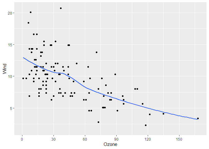
# More breaks

# get_breaks accepts a range too
gg +
  scale_x_continuous(breaks = \(x) get_breaks(range(x), 20))
#> `geom_smooth()` using method = 'loess' and formula = 'y ~ x'
#> Warning: Removed 37 rows containing non-finite outside the scale range
#> (`stat_smooth()`).
#> Removed 37 rows containing missing values or values outside the scale range
#> (`geom_point()`).