![]()
![]()
BayesERtools provides a suite of tools that facilitate
exposure-response analysis using Bayesian methods.
BayesERbook): https://genentech.github.io/BayesERbook/You can install the BayesERtools with:
install.packages('BayesERtools')
# devtools::install_github("genentech/BayesERtools") # development version|
Binary endpoint
|
Continuous endpoint
|
|||
|---|---|---|---|---|
| Linear (logit) | Emax (logit) | Linear | Emax | |
| backend |
rstanarm
|
rstanemax
|
rstanarm
|
rstanemax
|
| reference | 🔗 | 🔗 | 🔗 | 🔗 |
| develop model | ✅ | ✅ | ✅ | ✅ |
| simulate & plot ER | ✅ | ✅ | ✅ | ✅ |
| exposure metrics selection | ✅ | ✅ | ✅ | ✅ |
| covariate selection | ✅ | ❌ | ✅ | ❌ |
| covariate forest plot | ✅ | ❌ | ✅ | ❌ |
| ✅ Available, 🟡 In plan/under development, ❌ Not in a current plan | ||||
Here is a quick demo on how to use this package for E-R analysis. See Basic workflow for more thorough walk through.
# Load package and data
library(dplyr)
library(BayesERtools)
ggplot2::theme_set(ggplot2::theme_bw(base_size = 12))

data(d_sim_binom_cov)

# Hyperglycemia Grade 2+ (hgly2) data
df_er_ae_hgly2 <-
  d_sim_binom_cov |>
  filter(AETYPE == "hgly2") |>
  # Re-scale AUCss, baseline age
  mutate(
    AUCss_1000 = AUCss / 1000, BAGE_10 = BAGE / 10,
    Dose = paste(Dose_mg, "mg")
  )

var_resp <- "AEFLAG"set.seed(1234)
ermod_bin <- dev_ermod_bin(
data = df_er_ae_hgly2,
var_resp = var_resp,
var_exposure = "AUCss_1000"
)
ermod_bin
#>
#> ── Binary ER model ─────────────────────────────────────────────────────────────
#> ℹ Use `plot_er()` to visualize ER curve
#>
#> ── Developed model ──
#>
#> stan_glm
#> family: binomial [logit]
#> formula: AEFLAG ~ AUCss_1000
#> observations: 500
#> predictors: 2
#> ------
#> Median MAD_SD
#> (Intercept) -2.04 0.23
#> AUCss_1000 0.41 0.08
#> ------
#> * For help interpreting the printed output see ?print.stanreg
#> * For info on the priors used see ?prior_summary.stanreg
# Using `*` instead of `+` so that scale can be
# applied for both panels (main plot and boxplot)
plot_er_gof(ermod_bin, var_group = "Dose", show_coef_exp = TRUE) *
xgxr::xgx_scale_x_log10(guide = ggplot2::guide_axis(minor.ticks = TRUE))
#> Warning in ggplot2::annotate("label", x = pos_ci_annot[1], y = pos_ci_annot[2],
#> : Ignoring unknown parameters: `label.size`
#> Warning: annotation$theme is not a valid theme.
#> Please use `theme()` to construct themes.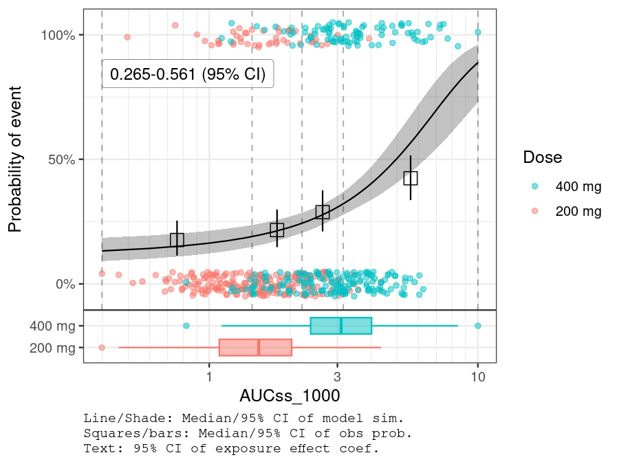
BGLUC (baseline glucose) is selected while other two covariates are not.
set.seed(1234)
ermod_bin_cov_sel <-
  dev_ermod_bin_cov_sel(
    data = df_er_ae_hgly2,
    var_resp = var_resp,
    var_exposure = "AUCss_1000",
    var_cov_candidate = c("BAGE_10", "RACE", "BGLUC")
  )
#>
#> ── Step 1: Full reference model fit ──
#>
#> ── Step 2: Variable selection ──
#>
#> ℹ The variables selected were: AUCss_1000, BGLUC
#>
#> ── Step 3: Final model fit ──
#>
#> ── Cov mod dev complete ──
#>
ermod_bin_cov_sel
#> ── Binary ER model & covariate selection ───────────────────────────────────────
#> ℹ Use `plot_submod_performance()` to see variable selection performance
#> ℹ Use `plot_er()` with `marginal = TRUE` to visualize marginal ER curve
#>
#> ── Selected model ──
#>
#> stan_glm
#>  family:       binomial [logit]
#>  formula:      AEFLAG ~ AUCss_1000 + BGLUC
#>  observations: 500
#>  predictors:   3
#> ------
#>             Median MAD_SD
#> (Intercept) -7.59   0.90
#> AUCss_1000   0.46   0.08
#> BGLUC        0.87   0.13
#> ------
#> * For help interpreting the printed output see ?print.stanreg
#> * For info on the priors used see ?prior_summary.stanreg
plot_submod_performance(ermod_bin_cov_sel)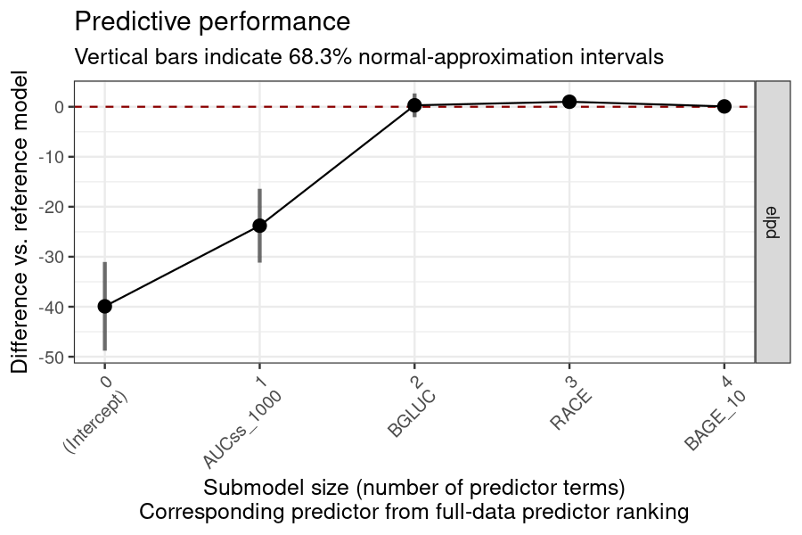
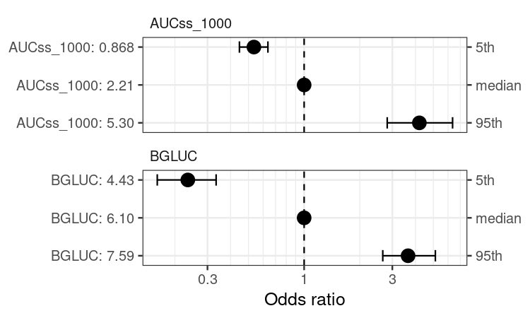
coveffsim <- sim_coveff(ermod_bin_cov_sel)
plot_coveff(coveffsim)
#> Warning in geom_errorbar(..., orientation = orientation): Ignoring unknown
#> parameters: `height`